How to Highlight Every Other Row in Google Sheets?

Table of Contents
Google Sheets can help reduce workload, bring a systematic approach, and increase productivity tenfold. This guide will explain how to highlight every other row in Google Sheets. If you are familiar with using Google Sheets, you probably would agree that it offers numerous features to make the work quick and easy. It has several formatting options and formulas that make handling massive data possible without confusion.
Alternating colors also add an aesthetic appeal when creating microcredentials. An online certificate looks much better when there is a color scheme differentiating scores or skills if you wish to highlight that in a tabular form.
Simple Steps to Alternate Colors in Google Sheets
Gone are the days when you had to check data or find an item in a 3,000-row list line by line. Not only that, but you can also combine first and last name in Excel without manually doing it. One formula is all it takes!
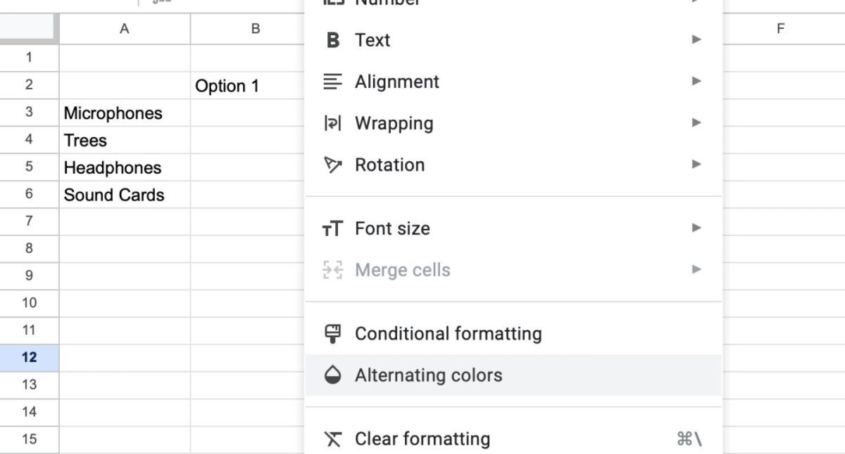
So, now to set alternate row colors in Excel, you have to select all the rows you want to format, select the ‘Format’ menu, click on ‘Alternating colors,’ and choose the color scheme you want to apply. Easy, no?
To simpler it even further, take a look at the below steps, with formulas, how to highlight every other row in Google Sheets:
- Select the whole data table you’ve created. You can do this either by click-dragging through the range of cells or by identifying the top and leftmost cell and then the bottom and rightmost cell.
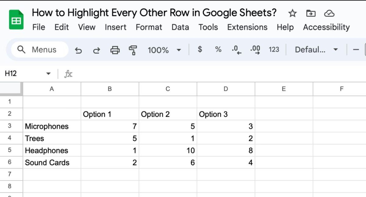
- Choose the FORMAT option. For this, go to the Home tab, select “Alternating colors” and pick a table style given there with alternate shading options.
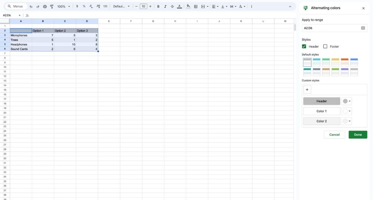
- The last step? Click Done, and voila, now you have a table with alternate colors.
Earlier, Google Sheets lacked several features that are present today. If you cannot find the options described above, it is likely because you are using an older version.
What’s the purpose of alternating colors in Google Sheets?

You might wonder why alternate colors in a table at all. Technically speaking, there is no need for color in a table; you don’t have to alternate them. But having said so, many organizations, firms, businesses, and institutions ask their staff or employees to use alternate colors when presenting data in tabular form. The foremost reason is to increase readability. Imagine 50 rows and columns of extensive data in table form. It will be challenging to read to keep track of where you left or started, no? When there are alternate colors in a table, reading it becomes considerably easy. And it also brings that aesthetic factor, which is critical in setting a professional image. Your presentation will look lively!
Choice of Colors in Google Sheets:
There may be times when you don’t want to use the default option. You want to experiment with other colors while creating a presentation or report for that WOW factor. Little changes and variations can bring out the presentation outstandingly. For instance, using creative fonts can also increase the readability and aesthetic appeal of a Google Sheet. There are 24+ best signature fonts in Word for you to use in Word.
So, here is what you can do:
Repeat the process! Select “alternating colors” in the “format option of the main menu. A sidebar labeled alternating colors will show up on the right side, with options for changing the colors of every other row.
You can select one of the default styles or manually choose color codes.
If you wish to select a custom color combo, all you have to do is click on the color pallet, which you can see just below the “alternate color” tab. The process is the same — select the range of the table you want to format, click the palette for each element, and pick the color.
What is Conditional Formatting?
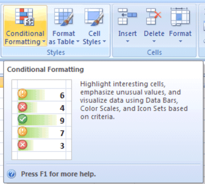
Those unfamiliar with the new Google Sheets version might very well know what conditional formatting is. It is a bit complicated, hands down, but if you memorize the formulas, alternating colors becomes quite simple.
How to highlight every other row in Google Sheets using conditional formatting?
Based on specific conditions, conditional formatting allows one to change row colors with default options, or you can even customize it.
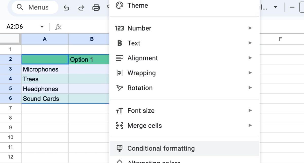
For changing colors with conditional formatting, go to the “Format” tab, select “Conditional formatting,” and specify your range. Once you do that, use the custom formula SEVEN(ROW()) for even rows. For odd rows, type =ISODD(ROW()). It will allow you to make a selection, and as you do so, you can pick colors from the color palette for custom selection. If not, select the entire table and choose a default alternate color option.
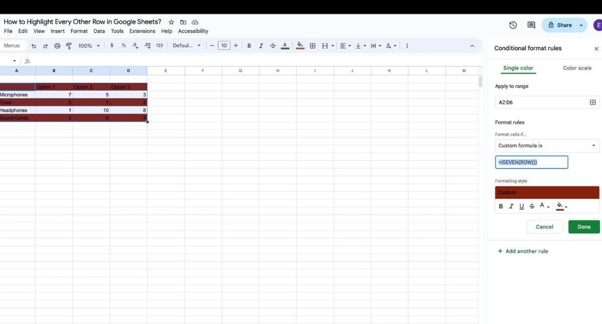
You can create elaborate row color patterns in Google Sheets with custom conditional formatting. You can apply several formulas to make the best use of this option.
For changing colors every third, fourth, or fifth row, however, you like, type MOD(ROW(), )=0. In this formula, you will see a space after the comma. In the space, you will type in a number, which implies the row you want to change the color for. For instance, MOD(ROW(),3)=0. The number 3 after the comma implies a color change on every third row. For alternating column colors, use =ISEVEN(COLUMN()) and =ISODD(COLUMN()).
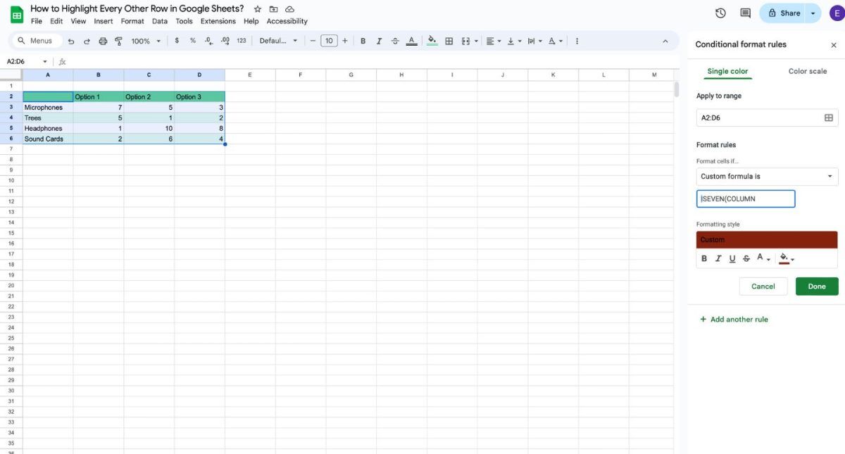
And we thought conditional formatting was difficult. 😃
Are rules for alternating row colors different in Excel and Google Sheets?
Not really! A slight variation may be, but that’s not rocket science. The general rules are the same for alternating colors; the only variation can be in formulas, a slight one, as Google Sheets keeps updating itself. And these syntaxes are easy to locate and find. So, no hassles!
However, using table settings in Excel is more direct and user-friendly for alternating row colors, particularly for beginners. But, for more advanced use, conditional formatting provides more room for customization. But for that, you’ll need a better understanding of formulas, to be direct, of advanced level.
You can also consider using a credential software. If you want to create a digital certificate with user details of tasks or the like in tabular form, such software helps lessen the burden. It gives you more time to focus on other things in a project.


